7.2 Three-Dimensional Graphics

The FriCAS three-dimensional graphics package provides the ability to graphics:three-dimensional

• generate surfaces defined by a function of two real variables
• generate space curves and tubes defined by parametric equations
• generate surfaces defined by parametric equations

These graphs can be modified by using various options, such as calculating points in the spherical coordinate system or changing the polygon grid size of a surface.

7.2.1 Plotting Three-Dimensional Functions of Two Variables

surface:two variable function The simplest three-dimensional graph is that of a surface defined by a function of two variables, z=f(x,y).

The general format for drawing a surface defined by a formula f(x,y) of two variables x and y is:

draw(f(x,y), x = a..b, y = c..d, options)

where a..b and c..d define the range of x and y, and where options

prescribes zero or more options as described in ugGraphThreeDOptions . An example of an option is title==”TitleofGraph”. An alternative format involving a function f is also available.

The simplest way to plot a function of two variables is to use a formula. With formulas you always precede the range specifications with the variable name and an = sign.

draw(cos(x*y),x=-3..3,y=-3..3)

If you intend to use a function more than once, or it is long and complex, then first give its definition to FriCAS.

f(x,y) == sin(x)*cos(y)

_{Type: Void}

To draw the function, just give its name and drop the variables from the range specifications. FriCAS compiles your function for efficient computation of data for the graph. Notice that FriCAS uses the text of your function as a default title.

draw(f,-%pi..%pi,-%pi..%pi)

7.2.2 Plotting Three-Dimensional Parametric Space Curves

A second kind of three-dimensional graph is a three-dimensional space curve curve:parametric space defined by the parametric equations for x(t), y(t), parametric space curve and z(t) as a function of an independent variable t.

The general format for drawing a three-dimensional space curve defined by parametric formulas x=f(t), y=g(t), and z=h(t) is:

draw(curve(f(t),g(t),h(t)), t = a..b, options)

where a..b defines the range of the independent variable t, and where

options prescribes zero or more options as described in ugGraphThreeDOptions . An example of an option is title==”TitleofGraph”. An alternative format involving functions f, g and h is also available.

If you use explicit formulas to draw a space curve, always precede the range specification with the variable name and an = sign.

draw(curve(5*cos(t), 5*sin(t),t), t=-12..12)

Alternatively, you can draw space curves by referring to functions.

i1(t:DFLOAT):DFLOAT == sin(t)*cos(3*t/5)

Function declaration i1 : DoubleFloat -> DoubleFloat has been added
   to workspace.

_{Type: Void}

This is useful if the functions are to be used more than once ...

i2(t:DFLOAT):DFLOAT == cos(t)*cos(3*t/5)

Function declaration i2 : DoubleFloat -> DoubleFloat has been added
   to workspace.

_{Type: Void}

or if the functions are long and complex.

i3(t:DFLOAT):DFLOAT == cos(t)*sin(3*t/5)

Function declaration i3 : DoubleFloat -> DoubleFloat has been added
   to workspace.

_{Type: Void}

Give the names of the functions and drop the variable name specification in the second argument. Again, FriCAS supplies a default title.

draw(curve(i1,i2,i3),0..15*%pi)

7.2.3 Plotting Three-Dimensional Parametric Surfaces

surface:parametric A third kind of three-dimensional graph is a surface defined by parametric surface parametric equations for x(u,v), y(u,v), and z(u,v) of two independent variables u and v.

The general format for drawing a three-dimensional graph defined by parametric formulas x=f(u,v), y=g(u,v), and z=h(u,v) is:

draw(surface(f(u,v),g(u,v),h(u,v)), u = a..b, v = c..d, options)

where a..b and c..d define the range of the independent variables u

and v, and where options prescribes zero or more options as described in ugGraphThreeDOptions . An example of an option is title==”TitleofGraph”. An alternative format involving functions f, g and h is also available.

This example draws a graph of a surface plotted using the parabolic cylindrical coordinate system option. coordinate system:parabolic cylindrical The values of the functions supplied to surface are parabolic cylindrical coordinate system interpreted in coordinates as given by a coordinates option, here as parabolic cylindrical coordinates (see ugGraphCoord ).

draw(surface(u*cos(v), u*sin(v), v*cos(u)), u=-4..4, v=0..%pi, coordinates== parabolicCylindrical)

Again, you can graph these parametric surfaces using functions, if the functions are long and complex.

Here we declare the types of arguments and values to be of type DoubleFloat.

n1(u:DFLOAT,v:DFLOAT):DFLOAT == u*cos(v)

Function declaration n1 : DoubleFloat -> DoubleFloat has been added
   to workspace.

_{Type: Void}

As shown by previous examples, these declarations are necessary.

n2(u:DFLOAT,v:DFLOAT):DFLOAT == u*sin(v)

Function declaration n2 : DoubleFloat -> DoubleFloat has been added
   to workspace.

_{Type: Void}

In either case, FriCAS compiles the functions when needed to graph a result.

n3(u:DFLOAT,v:DFLOAT):DFLOAT == u

Function declaration n3 : DoubleFloat -> DoubleFloat has been added
   to workspace.

_{Type: Void}

Without these declarations, you have to suffix floats with @DFLOAT to get a DoubleFloat result. However, a call here with an unadorned float produces a DoubleFloat.

n3(0.5,1.0)

Compiling function n3 with type (DoubleFloat,DoubleFloat) ->
   DoubleFloat

_{Type: DoubleFloat}

Draw the surface by referencing the function names, this time choosing the toroidal coordinate system. coordinate system:toroidal toroidal coordinate system

draw(surface(n1,n2,n3), 1..4, 1..2*%pi, coordinates == toroidal(1$DFLOAT))

7.2.4 Three-Dimensional Options

graphics:3D options The draw commands optionally take an optional list of options such as coordinates as shown in the last example. Each option is given by the syntax: name == value. Here is a list of the available options in the order that they are described below:

title	coordinates	var1Steps
style	tubeRadius	var2Steps
colorFunction	tubePoints	space

The option title gives your graph a title. graphics:3D options:title

draw(cos(x*y),x=0..2*%pi,y=0..%pi,title == “Title of Graph”)

The style determines which of four rendering algorithms is used for rendering the graph. The choices are “wireMesh”, “solid”, “shade”, and “smooth”.

draw(cos(x*y),x=-3..3,y=-3..3, style==”smooth”, title==”Smooth Option”)

In all but the wire-mesh style, polygons in a surface or tube plot are normally colored in a graph according to their z-coordinate value. Space curves are colored according to their parametric variable value. graphics:3D options:color function To change this, you can give a coloring function. function:coloring The coloring function is sampled across the range of its arguments, then normalized onto the standard FriCAS colormap.

A function of one variable makes the color depend on the value of the parametric variable specified for a tube plot.

color1(t) == t

_{Type: Void}

draw(curve(sin(t), cos(t),0), t=0..2*%pi, tubeRadius == .3, colorFunction == color1)

A function of two variables makes the color depend on the values of the independent variables.

color2(u,v) == u^2 - v^2

_{Type: Void}

Use the option colorFunction for special coloring.

draw(cos(u*v), u=-3..3, v=-3..3, colorFunction == color2)

With a three variable function, the color also depends on the value of the function.

color3(x,y,fxy) == sin(x*fxy) + cos(y*fxy)

_{Type: Void}

draw(cos(x*y), x=-3..3, y=-3..3, colorFunction == color3)

Normally the Cartesian coordinate system is used. Cartesian:coordinate system To change this, use the coordinates option. coordinate system:Cartesian For details, see ugGraphCoord .

m(u:DFLOAT,v:DFLOAT):DFLOAT == 1

Function declaration m : (DoubleFloat,DoubleFloat) -> DoubleFloat
   has been added to workspace.

_{Type: Void}

Use the spherical spherical coordinate system coordinate system. coordinate system:spherical

draw(m, 0..2*%pi,0..%pi, coordinates == spherical, style==”shade”)

Space curves may be displayed as tubes with polygonal cross sections. tube Two options, tubeRadius and tubePoints, control the size and shape of this cross section.

The tubeRadius option specifies the radius of the tube that tube:radius encircles the specified space curve.

draw(curve(sin(t),cos(t),0),t=0..2*%pi, style==”shade”, tubeRadius == .3)

The tubePoints option specifies the number of vertices tube:points in polygon defining the polygon that is used to create a tube around the specified space curve. The larger this number is, the more cylindrical the tube becomes.

draw(curve(sin(t), cos(t), 0), t=0..2*%pi, style==”shade”, tubeRadius == .25, tubePoints == 3)

graphics:3D options:variable steps

Options var1Stepsvar1StepsDrawOption and var2Stepsvar2StepsDrawOption specify the number of intervals into which the grid defining a surface plot is subdivided with respect to the first and second parameters of the surface function(s).

draw(cos(x*y),x=-3..3,y=-3..3, style==”shade”, var1Steps == 30, var2Steps == 30)

The space option of a draw command lets you build multiple graphs in three space. To use this option, first create an empty three-space object, then use the space option thereafter. There is no restriction as to the number or kinds of graphs that can be combined this way.

Create an empty three-space object.

s := create3Space()$(ThreeSpace DFLOAT)

\[\]

3-Spacewith0components

_{Type: ThreeSpace DoubleFloat}

m(u:DFLOAT,v:DFLOAT):DFLOAT == 1

Function declaration m : (DoubleFloat,DoubleFloat) -> DoubleFloat
   has been added to workspace.

_{Type: Void}

Add a graph to this three-space object. The new graph destructively inserts the graph into s.

draw(m,0..%pi,0..2*%pi, coordinates == spherical, space == s)

Add a second graph to s.

v := draw(curve(1.5*sin(t), 1.5*cos(t),0), t=0..2*%pi, tubeRadius == .25, space == s)

A three-space object can also be obtained from an existing three-dimensional viewport using the subspacesubspaceThreeSpace command. You can then use makeViewport3D to create a viewport window.

Assign to subsp the three-space object in viewport v.

subsp := subspace v

Reset the space component of v to the value of subsp.

subspace(v, subsp)

Create a viewport window from a three-space object.

makeViewport3D(subsp,”Graphs”)

7.2.5 The makeObject Command

An alternate way to create multiple graphs is to use makeObject. The makeObject command is similar to the draw command, except that it returns a three-space object rather than a ThreeDimensionalViewport. In fact, makeObject is called by the draw command to create the ThreeSpace then makeViewport3DmakeViewport3DThreeDimensionalViewport to create a viewport window.

m(u:DFLOAT,v:DFLOAT):DFLOAT == 1

Function declaration m : (DoubleFloat,DoubleFloat) -> DoubleFloat
   has been added to workspace.

_{Type: Void}

Do the last example a new way. First use makeObject to create a three-space object sph.

sph := makeObject(m, 0..%pi, 0..2*%pi, coordinates==spherical)

Compiling function m with type (DoubleFloat,DoubleFloat) ->
   DoubleFloat

\[\]

3-Spacewith1component

_{Type: ThreeSpace DoubleFloat}

Add a second object to sph.

makeObject(curve(1.5*sin(t), 1.5*cos(t), 0), t=0..2*%pi, space ==

sph, tubeRadius == .25)

Compiling function %D with type DoubleFloat -> DoubleFloat
Compiling function %F with type DoubleFloat -> DoubleFloat
Compiling function %H with type DoubleFloat -> DoubleFloat

\[\]

3-Spacewith2components

_{Type: ThreeSpace DoubleFloat}

Create and display a viewport containing sph.

makeViewport3D(sph,”Multiple Objects”)

Note that an undefined ThreeSpace parameter declared in a makeObject or draw command results in an error. Use the create3Spacecreate3SpaceThreeSpace function to define a ThreeSpace, or obtain a ThreeSpace that has been previously generated before including it in a command line.

7.2.6 Building Three-Dimensional Objects From Primitives

Rather than using the draw and makeObject commands, graphics:advanced:build 3D objects you can create three-dimensional graphs from primitives. Operation create3Spacecreate3SpaceThreeSpace creates a three-space object to which points, curves and polygons can be added using the operations from the ThreeSpace domain. The resulting object can then be displayed in a viewport using makeViewport3DmakeViewport3DThreeDimensionalViewport.

Create the empty three-space object space.

space := create3Space()$(ThreeSpace DFLOAT)

\[\]

3-Spacewith0components

_{Type: ThreeSpace DoubleFloat}

Objects can be sent to this space using the operations exported by the ThreeSpace domain. ThreeSpace The following examples place curves into space.

Add these eight curves to the space.

closedCurve(space,[ [0,30,20], [0,30,30], [0,40,30], [0,40,100],

[0,30,100],[0,30,110], [0,60,110], [0,60,100], [0,50,100], [0,50,30], [0,60,30], [0,60,20] ])

\[\]

3-Spacewith1component

_{Type: ThreeSpace DoubleFloat}

closedCurve(space,[ [80,0,30], [80,0,100], [70,0,110], [40,0,110],

[30,0,100], [30,0,90], [40,0,90], [40,0,95], [45,0,100], [65,0,100], [70,0,95], [70,0,35] ])

\[\]

3-Spacewith2components

_{Type: ThreeSpace DoubleFloat}

closedCurve(space,[ [70,0,35], [65,0,30], [45,0,30], [40,0,35],

[40,0,60], [50,0,60], [50,0,70], [30,0,70], [30,0,30], [40,0,20], [70,0,20], [80,0,30] ])

\[\]

3-Spacewith3components

_{Type: ThreeSpace DoubleFloat}

closedCurve(space,[ [0,70,20], [0,70,110], [0,110,110], [0,120,100],

[0,120,70], [0,115,65], [0,120,60], [0,120,30], [0,110,20], [0,80,20], [0,80,30], [0,80,20] ])

\[\]

3-Spacewith4components

_{Type: ThreeSpace DoubleFloat}

closedCurve(space,[ [0,105,30], [0,110,35], [0,110,55], [0,105,60],

[0,80,60], [0,80,70], [0,105,70], [0,110,75], [0,110,95], [0,105,100], [0,80,100], [0,80,20], [0,80,30] ])

\[\]

3-Spacewith5components

_{Type: ThreeSpace DoubleFloat}

closedCurve(space,[ [140,0,20], [140,0,110], [130,0,110], [90,0,20],

[101,0,20],[114,0,50], [130,0,50], [130,0,60], [119,0,60], [130,0,85], [130,0,20] ])

\[\]

3-Spacewith6components

_{Type: ThreeSpace DoubleFloat}

closedCurve(space,[ [0,140,20], [0,140,110], [0,150,110], [0,170,50],

[0,190,110], [0,200,110], [0,200,20], [0,190,20], [0,190,75], [0,175,35], [0,165,35],[0,150,75], [0,150,20] ])

\[\]

3-Spacewith7components

_{Type: ThreeSpace DoubleFloat}

closedCurve(space,[ [200,0,20], [200,0,110], [189,0,110], [160,0,45],

[160,0,110], [150,0,110], [150,0,20], [161,0,20], [190,0,85], [190,0,20] ])

\[\]

3-Spacewith8components

_{Type: ThreeSpace DoubleFloat}

Create and display the viewport using makeViewport3D. Options may also be given but here are displayed as a list with values enclosed in parentheses.

makeViewport3D(space, title == “Letters”)

7.2.6.1 Cube Example

As a second example of the use of primitives, we generate a cube using a polygon mesh. It is important to use a consistent orientation of the polygons for correct generation of three-dimensional objects.

Again start with an empty three-space object.

spaceC := create3Space()$(ThreeSpace DFLOAT)

\[\]

3-Spacewith0components

_{Type: ThreeSpace DoubleFloat}

For convenience, give DoubleFloat values +1 and -1 names.

x: DFLOAT := 1

\[\]

1.0

_{Type: DoubleFloat}

y: DFLOAT := -1

\[\]

-1.0

_{Type: DoubleFloat}

Define the vertices of the cube.

a := point [x,x,y,1::DFLOAT]$(Point DFLOAT)

\[\]

[1.0,1.0,-1.0,1.0]

_{Type: Point DoubleFloat}

b := point [y,x,y,4::DFLOAT]$(Point DFLOAT)

\[\]

[-1.0,1.0,-1.0,4.0]

_{Type: Point DoubleFloat}

c := point [y,x,x,8::DFLOAT]$(Point DFLOAT)

\[\]

[-1.0,1.0,1.0,8.0]

_{Type: Point DoubleFloat}

d := point [x,x,x,12::DFLOAT]$(Point DFLOAT)

\[\]

[1.0,1.0,1.0,12.0]

_{Type: Point DoubleFloat}

e := point [x,y,y,16::DFLOAT]$(Point DFLOAT)

\[\]

[1.0,-1.0,-1.0,16.0]

_{Type: Point DoubleFloat}

f := point [y,y,y,20::DFLOAT]$(Point DFLOAT)

\[\]

[-1.0,-1.0,-1.0,20.0]

_{Type: Point DoubleFloat}

g := point [y,y,x,24::DFLOAT]$(Point DFLOAT)

\[\]

[-1.0,-1.0,1.0,24.0]

_{Type: Point DoubleFloat}

h := point [x,y,x,27::DFLOAT]$(Point DFLOAT)

\[\]

[1.0,-1.0,1.0,27.0]

_{Type: Point DoubleFloat}

Add the faces of the cube as polygons to the space using a consistent orientation.

polygon(spaceC,[d,c,g,h])

\[\]

3-Spacewith1component

_{Type: ThreeSpace DoubleFloat}

polygon(spaceC,[d,h,e,a])

\[\]

3-Spacewith2components

_{Type: ThreeSpace DoubleFloat}

polygon(spaceC,[c,d,a,b])

\[\]

3-Spacewith3components

_{Type: ThreeSpace DoubleFloat}

polygon(spaceC,[g,c,b,f])

\[\]

3-Spacewith4components

_{Type: ThreeSpace DoubleFloat}

polygon(spaceC,[h,g,f,e])

\[\]

3-Spacewith5components

_{Type: ThreeSpace DoubleFloat}

polygon(spaceC,[e,f,b,a])

\[\]

3-Spacewith6components

_{Type: ThreeSpace DoubleFloat}

Create and display the viewport.

makeViewport3D(spaceC, title == “Cube”)

7.2.7 Coordinate System Transformations

graphics:advanced:coordinate systems

The CoordinateSystems package provides coordinate transformation functions that map a given data point from the coordinate system specified into the Cartesian coordinate system. CoordinateSystems The default coordinate system, given a triplet (f(u,v),u,v), assumes that z=f(u,v), x=u and y=v, that is, reads the coordinates in (z,x,y) order.

m(u:DFLOAT,v:DFLOAT):DFLOAT == u^2

Function declaration m : (DoubleFloat,DoubleFloat) -> DoubleFloat
   has been added to workspace.

_{Type: Void}

Graph plotted in default coordinate system.

draw(m,0..3,0..5)

The z coordinate comes first since the first argument of the draw command gives its values. In general, the coordinate systems FriCAS provides, or any that you make up, must provide a map to an (x,y,z) triplet in order to be compatible with the coordinatescoordinatesDrawOption DrawOption. DrawOption Here is an example.

Define the identity function.

cartesian(point:Point DFLOAT):Point DFLOAT == point

Function declaration cartesian : Point DoubleFloat -> Point
   DoubleFloat has been added to workspace.

_{Type: Void}

Pass cartesian as the coordinatescoordinatesDrawOption parameter to the draw command.

draw(m,0..3,0..5,coordinates==cartesian)

What happened? The option coordinates == cartesian directs FriCAS to treat the dependent variable m defined by m=u2 as the x coordinate. Thus the triplet of values (m,u,v) is transformed to coordinates (x,y,z) and so we get the graph of x=y2.

Here is another example. The cylindricalcylindricalCoordinateSystems transform takes coordinate system:cylindrical input of the form (w,u,v), interprets it in the order cylindrical coordinate system ( r, θ, z) and maps it to the Cartesian coordinates x=rcos(θ), y=rsin(θ), z=z in which r is the radius, θ is the angle and z is the z-coordinate.

An example using the cylindricalcylindricalCoordinateSystems coordinates for the constant r=3.

f(u:DFLOAT,v:DFLOAT):DFLOAT == 3

Function declaration f : (DoubleFloat,DoubleFloat) -> DoubleFloat
   has been added to workspace.

_{Type: Void}

Graph plotted in cylindrical coordinates.

draw(f,0..%pi,0..6,coordinates==cylindrical)

Suppose you would like to specify z as a function of r and θ instead of just r? Well, you still can use the cylindrical FriCAS transformation but we have to reorder the triplet before passing it to the transformation.

First, let’s create a point to work with and call it pt with some color col.

col := 5

\[\]

5

_{Type: PositiveInteger}

pt := point[1,2,3,col]$(Point DFLOAT)

\[\]

[1.0,2.0,3.0,5.0]

_{Type: Point DoubleFloat}

The reordering you want is (z,r,θ) to (r,θ,z) so that the first element is moved to the third element, while the second and third elements move forward and the color element does not change.

Define a function reorder to reorder the point elements.

reorder(p:Point DFLOAT):Point DFLOAT == point[p.2, p.3, p.1, p.4]

Function declaration reorder : Point DoubleFloat -> Point
   DoubleFloat has been added to workspace.

_{Type: Void}

The function moves the second and third elements forward but the color does not change.

reorder pt

\[\]

[2.0,3.0,1.0,5.0]

_{Type: Point DoubleFloat}

The function newmap converts our reordered version of the cylindrical coordinate system to the standard (x,y,z) Cartesian system.

newmap(pt:Point DFLOAT):Point DFLOAT == cylindrical(reorder pt)

Function declaration newmap : Point DoubleFloat -> Point DoubleFloat
   has been added to workspace.

_{Type: Void}

newmap pt

\[\]

[-1.9799849932008908,0.28224001611973443,1.0,5.0]

_{Type: Point DoubleFloat}

Graph the same function f using the coordinate mapping of the function newmap, so it is now interpreted as z=3:

draw(f,0..3,0..2*%pi,coordinates==newmap)

The CoordinateSystems package exports the following coordinate system operations: bipolar, bipolarCylindrical, cartesian, conical, cylindrical, elliptic, ellipticCylindrical, oblateSpheroidal, parabolic, parabolicCylindrical, paraboloidal, polar, prolateSpheroidal, spherical, and toroidal. Use Browse or the )show system command show to get more information.

7.2.8 Three-Dimensional Clipping

A three-dimensional graph can be explicitly clipped within the draw graphics:advanced:clip command by indicating a minimum and maximum threshold for the clipping given function definition. These thresholds can be defined using the FriCAS min and max functions.

gamma(x,y) ==
  g := Gamma complex(x,y)
  point [x, y, max( min(real g, 4), -4), argument g]

Here is an example that clips the gamma function in order to eliminate the extreme divergence it creates.

draw(gamma,-%pi..%pi,-%pi..%pi,var1Steps==50,var2Steps==50)

7.2.9 Three-Dimensional Control-Panel

graphics:3D control-panel Once you have created a viewport, move your mouse to the viewport and click with your left mouse button. This displays a control-panel on the side of the viewport that is closest to where you clicked.

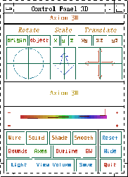
Three-dimensional control-panel.

7.2.9.1 Transformations

We recommend you first select the Bounds button while graphics:3D control-panel:transformations executing transformations since the bounding box displayed indicates the object’s position as it changes.

Rotate:

A rotation transformation occurs by clicking the mouse graphics:3D control-panel:rotate within the Rotate window in the upper left corner of the control-panel. The rotation is computed in spherical coordinates, using the horizontal mouse position to increment or decrement the value of the longitudinal angle θ within the range of 0 to 2 π and the vertical mouse position to increment or decrement the value of the latitudinal angle within the range of - π to π. The active mode of rotation is displayed in green on a color monitor or in clear text on a black and white monitor, while the inactive mode is displayed in red for color display or a mottled pattern for black and white.

origin:

The origin button indicates that the rotation is to occur with respect to the origin of the viewing space, that is indicated by the axes.

object:

The object button indicates that the rotation is to occur with respect to the center of volume of the object, independent of the axes’ origin position.

Scale:

A scaling transformation occurs by clicking the mouse graphics:3D control-panel:scale within the Scale window in the upper center of the control-panel, containing a zoom arrow. The axes along which the scaling is to occur are indicated by selecting the appropriate button above the zoom arrow window. The selected axes are displayed in green on a color monitor or in clear text on a black and white monitor, while the unselected axes are displayed in red for a color display or a mottled pattern for black and white.

uniform:

Uniform scaling along the x, y and z axes occurs when all the axes buttons are selected.

non-uniform:

If any of the axes buttons are not selected, non-uniform scaling occurs, that is, scaling occurs only in the direction of the axes that are selected.

Translate:

Translation occurs by indicating with the mouse in the graphics:3D control-panel:translate Translate window the direction you want the graph to move. This window is located in the upper right corner of the control-panel and contains a potentiometer with crossed arrows pointing up, down, left and right. Along the top of the Translate window are three buttons ( XY, XZ, and YZ) indicating the three orthographic projection planes. Each orientates the group as a view into that plane. Any translation of the graph occurs only along this plane.

7.2.9.2 Messages

graphics:3D control-panel:messages

The window directly below the potentiometer windows for transformations is used to display system messages relating to the viewport, the control-panel and the current graph displaying status.

7.2.9.3 Colormap

graphics:3D control-panel:color map

Directly below the message window is the colormap range indicator window. colormap The FriCAS Colormap shows a sampling of the spectrum from which hues can be drawn to represent the colors of a surface. The Colormap is composed of five shades for each of the hues along this spectrum. By moving the markers above and below the Colormap, the range of hues that are used to color the existing surface are set. The bottom marker shows the hue for the low end of the color range and the top marker shows the hue for the upper end of the range. Setting the bottom and top markers at the same hue results in monochromatic smooth shading of the graph when Smooth mode is selected. At each end of the Colormap are + and - buttons. When clicked on, these increment or decrement the top or bottom marker.

7.2.9.4 Buttons

graphics:3D control-panel:buttons

Below the Colormap window and to the left are located various buttons that determine the characteristics of a graph. The buttons along the bottom and right hand side all have special meanings; the remaining buttons in the first row indicate the mode or style used to display the graph. The second row are toggles that turn on or off a property of the graph. On a color monitor, the property is on if green (clear text, on a monochrome monitor) and off if red (mottled pattern, on a monochrome monitor). Here is a list of their functions.

Wire

displays surface and tube plots as a graphics:3D control-panel:wire wireframe image in a single color (blue) with no hidden surfaces removed, or displays space curve plots in colors based upon their parametric variables. This is the fastest mode for displaying a graph. This is very useful when you want to find a good orientation of your graph.

Solid

displays the graph with hidden graphics:3D control-panel:solid surfaces removed, drawing each polygon beginning with the furthest from the viewer. The edges of the polygons are displayed in the hues specified by the range in the Colormap window.

Shade

displays the graph with hidden graphics:3D control-panel:shade surfaces removed and with the polygons shaded, drawing each polygon beginning with the furthest from the viewer. Polygons are shaded in the hues specified by the range in the Colormap window using the Phong illumination model. Phong:illumination model

Smooth

displays the graph using a graphics:3D control-panel:smooth renderer that computes the graph one line at a time. The location and color of the graph at each visible point on the screen are determined and displayed using the Phong illumination Phong:illumination model model. Smooth shading is done in one of two ways, depending on the range selected in the colormap window and the number of colors available from the hardware and/or window manager. When the top and bottom markers of the colormap range are set to different hues, the graph is rendered by dithering between the dithering transitions in color hue. When the top and bottom markers of the colormap range are set to the same hue, the graph is rendered using the Phong smooth shading model. Phong:smooth shading model However, if enough colors cannot be allocated for this purpose, the renderer reverts to the color dithering method until a sufficient color supply is available. For this reason, it may not be possible to render multiple Phong smooth shaded graphs at the same time on some systems.

Bounds

encloses the entire volume of the viewgraph within a bounding box, or removes the box if previously selected. graphics:3D control-panel:bounds The region that encloses the entire volume of the viewport graph is displayed.

Axes

displays Cartesian graphics:3D control-panel:axes coordinate axes of the space, or turns them off if previously selected.

Outline

causes graphics:3D control-panel:outline quadrilateral polygons forming the graph surface to be outlined in black when the graph is displayed in Shade mode.

BW

converts a color viewport to black and white, or vice-versa. graphics:3D control-panel:bw When this button is selected the control-panel and viewport switch to an immutable colormap composed of a range of grey scale patterns or tiles that are used wherever shading is necessary.

Light

takes you to a control-panel described below.

ViewVolume

takes you to another control-panel as described below. graphics:3D control-panel:save

Save

creates a menu of the possible file types that can be written using the control-panel. The Exit button leaves the save menu. The Pixmap button writes an FriCAS pixmap of graphics:3D control-panel:pixmap the current viewport contents. The file is called axiom3D.pixmap and is located in the directory from which FriCAS or viewAlone was started. The PS button writes the current viewport contents to graphics:3D control-panel:ps PostScript output rather than to the viewport window. By default the file is called axiom3D.ps; however, if a file file:.Xdefaults @ .Xdefaults name is specified in the user’s .Xdefaults file it is graphics:.Xdefaults:PostScript file name used. The file is placed in the directory from which the FriCAS or viewAlone session was begun. See also the writewriteThreeDimensionalViewport function. PostScript

Reset

returns the object transformation graphics:3D control-panel:reset characteristics back to their initial states.

Hide

causes the control-panel for the graphics:3D control-panel:hide corresponding viewport to disappear from the screen.

Quit

queries whether the current viewport graphics:3D control-panel:quit session should be terminated.

7.2.9.5 Light

graphics:3D control-panel:light

The Light button changes the control-panel into the Lighting Control-Panel. At the top of this panel, the three axes are shown with the same orientation as the object. A light vector from the origin of the axes shows the current position of the light source relative to the object. At the bottom of the panel is an Abort button that cancels any changes to the lighting that were made, and a Return button that carries out the current set of lighting changes on the graph.

XY:

The XY lighting axes window is below the graphics:3D control-panel:move xy Lighting Control-Panel title and to the left. This changes the light vector within the XY view plane.

Z:

The Z lighting axis window is below the graphics:3D control-panel:move z Lighting Control-Panel title and in the center. This changes the Z location of the light vector.

Intensity:

Below the Lighting Control-Panel title graphics:3D control-panel:intensity and to the right is the light intensity meter. Moving the intensity indicator down decreases the amount of light emitted from the light source. When the indicator is at the top of the meter the light source is emitting at 100% intensity. At the bottom of the meter the light source is emitting at a level slightly above ambient lighting.

7.2.9.6 View Volume

graphics:3D control-panel:view volume

The View Volume button changes the control-panel into the Viewing Volume Panel. At the bottom of the viewing panel is an Abort button that cancels any changes to the viewing volume that were made and a Return button that carries out the current set of viewing changes to the graph.

Eye Reference:

At the top of this panel is the graphics:3D control-panel:eye reference Eye Reference window. It shows a planar projection of the viewing pyramid from the eye of the viewer relative to the location of the object. This has a bounding region represented by the rectangle on the left. Below the object rectangle is the Hither window. By moving the slider in this window the hither clipping plane sets hither clipping plane the front of the view volume. As a result of this depth clipping all points of the object closer to the eye than this hither plane are not shown. The Eye Distance slider to the right of the Hither slider is used to change the degree of perspective in the image.

Clip Volume:

The Clip Volume window is at the graphics:3D control-panel:clip volume bottom of the Viewing Volume Panel. On the right is a Settings menu. In this menu are buttons to select viewing attributes. Selecting the Perspective button computes the image using perspective projection. graphics:3D control-panel:perspective The Show Region button indicates whether the clipping region of the graphics:3D control-panel:show clip region volume is to be drawn in the viewport and the Clipping On button shows whether the view volume clipping is to be in effect when the image graphics:3D control-panel:clipping on is drawn. The left side of the Clip Volume window shows the clipping graphics:3D control-panel:clip volume boundary of the graph. Moving the knobs along the X, Y, and Z sliders adjusts the volume of the clipping region accordingly.

7.2.10 Operations for Three-Dimensional Graphics

Here is a summary of useful FriCAS operations for three-dimensional graphics. Each operation name is followed by a list of arguments. Each argument is written as a variable informally named according to the type of the argument (for example, integer). If appropriate, a default value for an argument is given in parentheses immediately following the name.

adaptive3D? ()

tests whether space curves are to be plotted graphics:plot3d defaults:adaptive according to the adaptive plotting adaptive refinement algorithm.

axes (viewport, string(“on”))

turns the axes on and off. graphics:3D commands:axes

close (viewport)

closes the viewport. graphics:3D commands:close

colorDef (viewport, color1(1), color2(27))

sets the colormap graphics:3D commands:define color range to be from color1 to color2.

controlPanel (viewport, string(“off”))

declares whether the graphics:3D commands:control-panel control-panel for the viewport is to be displayed or not.

diagonals (viewport, string(“off”))

declares whether the graphics:3D commands:diagonals polygon outline includes the diagonals or not.

drawStyle (viewport, style)

selects which of four drawing styles graphics:3D commands:drawing style are used: “wireMesh”, “solid”, “shade”, or “smooth”.

eyeDistance (viewport,float(500))

sets the distance of the eye from the origin of the object graphics:3D commands:eye distance for use in the perspectiveperspectiveThreeDimensionalViewport.

key (viewport)

returns the operating graphics:3D commands:key system process ID number for the viewport.

lighting (viewport, floatx(-0.5), floaty(0.5), floatz(0.5))

sets the Cartesian graphics:3D commands:lighting coordinates of the light source.

modifyPointData (viewport,integer,point)

replaces the coordinates of the point with graphics:3D commands:modify point data the index integer with point.

move (viewport, integerx(viewPosDefault), integery(viewPosDefault))

moves the upper graphics:3D commands:move left-hand corner of the viewport to screen position ({ integerx, integery}).

options (viewport)

returns a list of all current draw options.

outlineRender (viewport, string(“off”))

turns polygon outlining graphics:3D commands:outline off or on when drawing in “shade” mode.

perspective (viewport, string(“on”))

turns perspective graphics:3D commands:perspective viewing on and off.

reset (viewport)

resets the attributes of a viewport to their graphics:3D commands:reset initial settings.

resize (viewport, integerwidth (viewSizeDefault), integerheight

(viewSizeDefault))

resets the width and height graphics:3D commands:resize values for a viewport.

rotate (viewport, numberθ(viewThetaDefapult), (viewPhiDefault))

rotates the viewport by rotation angles for longitude ( θ) and latitude ( ). Angles designate radians if given as floats, or degrees if given graphics:3D commands:rotate as integers.

setAdaptive3D (boolean(true))

sets whether space curves are to be plotted graphics:plot3d defaults:set adaptive according to the adaptive adaptive plotting refinement algorithm.

setMaxPoints3D (integer(1000))

sets the default maximum number of possible graphics:plot3d defaults:set max points points to be used when constructing a three-dimensional space curve.

setMinPoints3D (integer(49))

sets the default minimum number of possible graphics:plot3d defaults:set min points points to be used when constructing a three-dimensional space curve.

setScreenResolution3D (integer(49))

sets the default screen resolution constant graphics:plot3d defaults:set screen resolution used in setting the computation limit of adaptively adaptive plotting generated three-dimensional space curve plots.

showRegion (viewport, string(“off”))

declares whether the bounding graphics:3D commands:showRegion box of a graph is shown or not.

subspace (viewport)

returns the space component.

subspace (viewport, subspace)

resets the space component graphics:3D commands:subspace to subspace.

title (viewport, string)

gives the viewport the graphics:3D commands:title title string.

translate (viewport, floatx(viewDeltaXDefault),

floaty(viewDeltaYDefault))

translates graphics:3D commands:translate the object horizontally and vertically relative to the center of the viewport.

intensity (viewport,float(1.0))

resets the intensity I of the light source, graphics:3D commands:intensity 0≤I≤1.

tubePointsDefault ([integer(6)])

sets or indicates the default number of graphics:3D defaults:tube points vertices defining the polygon that is used to create a tube around a space curve.

tubeRadiusDefault ([float(0.5)])

sets or indicates the default radius of graphics:3D defaults:tube radius the tube that encircles a space curve.

var1StepsDefault ([integer(27)])

sets or indicates the default number of graphics:3D defaults:var1 steps increments into which the grid defining a surface plot is subdivided with respect to the first parameter declared in the surface function.

var2StepsDefault ([integer(27)])

sets or indicates the default number of graphics:3D defaults:var2 steps increments into which the grid defining a surface plot is subdivided with respect to the second parameter declared in the surface function.

viewDefaults ([ integerpoint, integerline, integeraxes, integerunits,

floatpoint, listposition, listsize])

resets the default settings for the graphics:3D defaults:reset viewport defaults point color, line color, axes color, units color, point size, viewport upper left-hand corner position, and the viewport size.

viewDeltaXDefault ([float(0)])

resets the default horizontal offset graphics:3D commands:deltaX default from the center of the viewport, or returns the current default offset if no argument is given.

viewDeltaYDefault ([float(0)])

resets the default vertical offset graphics:3D commands:deltaY default from the center of the viewport, or returns the current default offset if no argument is given.

viewPhiDefault ([float(- π/4)])

resets the default latitudinal view angle, or returns the current default angle if no argument is given. graphics:3D commands:phi default is set to this value.

viewpoint (viewport, floatx, floaty, floatz)

sets the viewing position in Cartesian coordinates.

viewpoint (viewport, floatθ, )

sets the viewing position in spherical coordinates.

viewpoint (viewport, Floatθ, , FloatscaleFactor, FloatxOffset,

FloatyOffset)

sets the viewing position in spherical coordinates, the scale factor, and offsets. graphics:3D commands:viewpoint θ (longitude) and (latitude) are in radians.

viewPosDefault ([list([0,0])])

sets or indicates the position of the upper graphics:3D defaults:viewport position left-hand corner of a two-dimensional viewport, relative to the display root window (the upper left-hand corner of the display is [0,0]).

viewSizeDefault ([list([400,400])])

sets or indicates the width and height dimensions graphics:3D defaults:viewport size of a viewport.

viewThetaDefault ([float( π/4)])

resets the default longitudinal view angle, or returns the current default angle if no argument is given. graphics:3D commands:theta default When a parameter is specified, the default longitudinal view angle θ is set to this value.

viewWriteAvailable ([list([“pixmap”, “bitmap”, “postscript”,

“image”])])

indicates the possible file types graphics:3D defaults:available viewport writes that can be created with the writewriteThreeDimensionalViewport function.

viewWriteDefault ([list([])])

sets or indicates the default types of files that are created in addition to the data file when a writewriteThreeDimensionalViewport command graphics:3D defaults:viewport writes is executed on a viewport.

viewScaleDefault ([float])

sets the default scaling factor, or returns graphics:3D commands:scale default the current factor if no argument is given.

write (viewport, directory, [option])

writes the file data for viewport in the directory directory. An optional third argument specifies a file type (one of pixmap, bitmap, postscript, or image), or a list of file types. An additional file is written for each file type listed.

scale (viewport, float(2.5))

specifies the scaling factor. graphics:3D commands:scale scaling graphs

7.2.11 Customization using .Xdefaults

graphics:.Xdefaults

Both the two-dimensional and three-dimensional drawing facilities consult the .Xdefaults file for various defaults. file:.Xdefaults @ .Xdefaults The list of defaults that are recognized by the graphing routines is discussed in this section. These defaults are preceded by FriCAS.3D. for three-dimensional viewport defaults, FriCAS.2D. for two-dimensional viewport defaults, or FriCAS* (no dot) for those defaults that are acceptable to either viewport type.

FriCAS*buttonFont: font

This indicates which graphics:.Xdefaults:button font font type is

used for the button text on the control-panel. Rom11

FriCAS.2D.graphFont: font

  (2D only)

This indicates graphics:.Xdefaults:graph number font which font

type is used for displaying the graph numbers and slots in the Graphs section of the two-dimensional control-panel. Rom22

FriCAS.3D.headerFont: font

This indicates which graphics:.Xdefaults:graph label font font type

is used for the axes labels and potentiometer header names on three-dimensional viewport windows. This is also used for two-dimensional control-panels for indicating which font type is used for potentionmeter header names and multiple graph title headers. Itl14

FriCAS*inverse: switch

This indicates whether the graphics:.Xdefaults:inverting background

background color is to be inverted from white to black. If on, the graph viewports use black as the background color. If off or no declaration is made, the graph viewports use a white background. off

FriCAS.3D.lightingFont: font

  (3D only)

This indicates which font type is used for the x,

graphics:.Xdefaults:lighting font y, and z labels of the two lighting axes potentiometers, and for the Intensity title on the lighting control-panel. Rom10

FriCAS.2D.messageFont, FriCAS.3D.messageFont: font

These indicate the font type graphics:.Xdefaults:message font to be

used for the text in the control-panel message window. Rom14

FriCAS*monochrome: switch

This indicates whether the graphics:.Xdefaults:monochrome graph

viewports are to be displayed as if the monitor is black and white, that is, a 1 bit plane. If on is specified, the viewport display is black and white. If off is specified, or no declaration for this default is given, the viewports are displayed in the normal fashion for the monitor in use. off

FriCAS.2D.postScript: filename

This specifies graphics:.Xdefaults:PostScript file name the name of

the file that is generated when a 2D PostScript graph PostScript is saved. axiom2D.ps

FriCAS.3D.postScript: filename

This specifies graphics:.Xdefaults:PostScript file name the name of

the file that is generated when a 3D PostScript graph PostScript is saved. axiom3D.ps

FriCAS*titleFont font

This graphics:.Xdefaults:title font indicates which font type is

used for the title text and, for three-dimensional graphs, in the lighting and viewing-volume control-panel windows. graphics:Xdefaults:2d Rom14

FriCAS.2D.unitFont: font

  (2D only)

This indicates graphics:.Xdefaults:unit label font which font type

is used for displaying the unit labels on two-dimensional viewport graphs. 6x10

FriCAS.3D.volumeFont: font

  (3D only)

This indicates which font type is used for the x,

graphics:.Xdefaults:volume label font y, and z labels of the clipping region sliders; for the Perspective, Show Region, and Clipping On buttons under Settings, and above the windows for the Hither and Eye Distance sliders in the Viewing Volume Panel of the three-dimensional control-panel. Rom8